Dark Consequences (DATA Unit Files Book 2)

‘I made Steve Bannon’s psychological warfare tool’: meet the data war whistleblower

---

In Matplotlib, we do this by modifying the transform. Any graphics display framework needs some scheme for translating between coordinate systems. For example, a data point at needs to somehow be represented at a certain location on the figure, which in turn needs to be represented in pixels on the screen. Mathematically, such coordinate transformations are relatively straightforward, and Matplotlib has a well-developed set of tools that it uses internally to perform them the tools can be explored in the matplotlib. The average user rarely needs to worry about the details of these transforms, but it is helpful knowledge to have when considering the placement of text on a figure.

There are three predefined transforms that can be useful in this situation:.

The transData coordinates give the usual data coordinates associated with the x- and y-axis labels. The transAxes coordinates give the location from the bottom-left corner of the axes here the white box as a fraction of the axes size. The transFigure coordinates are similar, but specify the position from the bottom left of the figure here the gray box as a fraction of the figure size. Along with tick marks and text, another useful annotation mark is the simple arrow.

Drawing arrows in Matplotlib is often much harder than you might hope.

Resetting the Circadian Clock

While there is a plt. This function creates some text and an arrow, and the arrows can be very flexibly specified. The arrow style is controlled through the arrowprops dictionary, which has numerous options available. Unfortunately, it also means that these sorts of features often must be manually tweaked, a process that can be very time-consuming when one is producing publication-quality graphics!

More discussion and examples of available arrow and annotation styles can be found in the Matplotlib gallery , in particular http: Before we go into examples, it will be best for us to understand further the object hierarchy of Matplotlib plots. Matplotlib aims to have a Python object representing everything that appears on the plot: Each Matplotlib object can also act as a container of sub-objects; for example, each figure can contain one or more axes objects, each of which in turn contain other objects representing plot contents.

The tick marks are no exception. Each axes has attributes xaxis and yaxis , which in turn have attributes that contain all the properties of the lines, ticks, and labels that make up the axes. Within each axis, there is the concept of a major tick mark and a minor tick mark. As the names would imply, major ticks are usually bigger or more pronounced, while minor ticks are usually smaller. We see here that each major tick shows a large tick mark and a label, while each minor tick shows a smaller tick mark with no label.

We can customize these tick properties—that is, locations and labels—by setting the formatter and locator objects of each axis.

Free Books Download Online Pdf Dark Consequences Data Unit Files Volume 2 By Lexxie Scott Pdf Djvu

We see that both major and minor tick labels have their locations specified by a LogLocator which makes sense for a logarithmic plot. Minor ticks, though, have their labels formatted by a NullFormatter ; this says that no labels will be shown. We can do this using plt. Having no ticks at all can be useful in many situations—for example, when you want to show a grid of images. One common problem with the default settings is that smaller subplots can end up with crowded labels.

Particularly for the x ticks, the numbers nearly overlap, making them quite difficult to decipher. We can fix this with the plt. MaxNLocator , which allows us to specify the maximum number of ticks that will be displayed. This makes things much cleaner. If you want even more control over the locations of regularly spaced ticks, you might also use plt. There are a couple changes we might like to make. We can do this by setting a MultipleLocator , which locates ticks at a multiple of the number you provide.

But now these tick labels look a little bit silly: To fix this, we can change the tick formatter. This is much better! For more information on any of these, refer to the docstrings or to the Matplotlib online documentation. Each of the following is available in the plt namespace:. While much is slated to change in the 2. But this took a whole lot of effort! We definitely do not want to have to do all that tweaking each time we create a plot. Fortunately, there is a way to adjust these defaults once in a way that will work for all plots.

Each time Matplotlib loads, it defines a runtime configuration rc containing the default styles for every plot element you create. You can adjust this configuration at any time using the plt.

Missing the Dark: Health Effects of Light Pollution

I find this much more aesthetically pleasing than the default styling. If you disagree with my aesthetic sense, the good news is that you can adjust the rc parameters to suit your own tastes! These settings can be saved in a. That said, I prefer to customize Matplotlib using its stylesheets instead. These stylesheets are formatted similarly to the. The available styles are listed in plt.

But keep in mind that this will change the style for the rest of the session! Alternatively, you can use the style context manager, which sets a style temporarily:. The ggplot package in the R language is a very popular visualization tool. There is a very nice short online book called Probabilistic Programming and Bayesian Methods for Hackers ; it features figures created with Matplotlib, and uses a nice set of rc parameters to create a consistent and visually appealing style throughout the book. For figures used within presentations, it is often useful to have a dark rather than light background.

Sometimes you might find yourself preparing figures for a print publication that does not accept color figures. As we will see, these styles are loaded automatically when Seaborn is imported into a notebook. With all of these built-in options for various plot styles, Matplotlib becomes much more useful for both interactive visualization and creation of figures for publication. Throughout this book, I will generally use one or more of these style conventions when creating plots. Matplotlib was initially designed with only two-dimensional plotting in mind.

Around the time of the 1. With this 3D axes enabled, we can now plot a variety of three-dimensional plot types. The most basic three-dimensional plot is a line or scatter plot created from sets of x, y, z triples. In analogy with the more common two-dimensional plots discussed earlier, we can create these using the ax. Notice that by default, the scatter points have their transparency adjusted to give a sense of depth on the page.

While the three-dimensional effect is sometimes difficult to see within a static image, an interactive view can lead to some nice intuition about the layout of the points. Two other types of three-dimensional plots that work on gridded data are wireframes and surface plots. These take a grid of values and project it onto the specified three-dimensional surface, and can make the resulting three-dimensional forms quite easy to visualize.

A surface plot is like a wireframe plot, but each face of the wireframe is a filled polygon. Note that though the grid of values for a surface plot needs to be two-dimensional, it need not be rectilinear. For some applications, the evenly sampled grids required by the preceding routines are overly restrictive and inconvenient.

In these situations, the triangulation-based plots can be very useful. What if rather than an even draw from a Cartesian or a polar grid, we instead have a set of random draws? This leaves a lot to be desired. The function that will help us in this case is ax. The result is certainly not as clean as when it is plotted with a grid, but the flexibility of such a triangulation allows for some really interesting three-dimensional plots. Now from this parameterization, we must determine the x, y, z positions of the embedded strip.

Thinking about it, we might realize that there are two rotations happening: Now we use our recollection of trigonometry to derive the three-dimensional embedding. Finally, to plot the object, we must make sure the triangulation is correct. Combining all of these techniques, it is possible to create and display a wide variety of three-dimensional objects and patterns in Matplotlib. One common type of visualization in data science is that of geographic data. Admittedly, Basemap feels a bit clunky to use, and often even simple visualizations take much longer to render than you might hope.

More modern solutions, such as leaflet or the Google Maps API, may be a better choice for more intensive map visualizations. Still, Basemap is a useful tool for Python users to have in their virtual toolbelts. The useful thing is that the globe shown here is not a mere image; it is a fully functioning Matplotlib axes that understands spherical coordinates and allows us to easily over-plot data on the map! For example, we can use a different map projection, zoom in to North America, and plot the location of Seattle. This gives you a brief glimpse into the sort of geographic visualizations that are possible with just a few lines of Python.

Using these brief examples as building blocks, you should be able to create nearly any map visualization that you desire. The first thing to decide when you are using maps is which projection to use. These projections have been developed over the course of human history, and there are a lot of choices! Depending on the intended use of the map projection, there are certain map features e. The Basemap package implements several dozen such projections, all referenced by a short format code.

The simplest of map projections are cylindrical projections, in which lines of constant latitude and longitude are mapped to horizontal and vertical lines, respectively.

This type of mapping represents equatorial regions quite well, but results in extreme distortions near the poles. The spacing of latitude lines varies between different cylindrical projections, leading to different conservation properties, and different distortion near the poles. The additional arguments to Basemap for this view specify the latitude lat and longitude lon of the lower-left corner llcrnr and upper-right corner urcrnr for the desired map, in units of degrees.

Pseudo-cylindrical projections relax the requirement that meridians lines of constant longitude remain vertical; this can give better properties near the poles of the projection.

It is constructed so as to preserve area across the map: Perspective projections are constructed using a particular choice of perspective point, similar to if you photographed the Earth from a particular point in space a point which, for some projections, technically lies within the Earth! Thus, it can show only half the globe at a time. These are often the most useful for showing small portions of the map. A conic projection projects the map onto a single cone, which is then unrolled. This can lead to very good local properties, but regions far from the focus point of the cone may become very distorted.

Conic projections, like perspective projections, tend to be good choices for representing small to medium patches of the globe. Most likely, they are available in the Basemap package. Earlier we saw the bluemarble and shadedrelief methods for projecting global images on the map, as well as the drawparallels and drawmeridians methods for drawing lines of constant latitude and longitude.

The Basemap package contains a range of useful functions for drawing borders of physical features like continents, oceans, lakes, and rivers, as well as political boundaries such as countries and US states and counties. For the boundary-based features, you must set the desired resolution when creating a Basemap image.

The resolution argument of the Basemap class sets the level of detail in boundaries, either 'c' crude , 'l' low , 'i' intermediate , 'h' high , 'f' full , or None if no boundaries will be used. This choice is important: Notice that the low-resolution coastlines are not suitable for this level of zoom, while high-resolution works just fine. The low level would work just fine for a global view, however, and would be much faster than loading the high-resolution border data for the entire globe! It might require some experimentation to find the correct resolution parameter for a given view; the best route is to start with a fast, low-resolution plot and increase the resolution as needed.

Perhaps the most useful piece of the Basemap toolkit is the ability to over-plot a variety of data onto a map background. For simple plotting and text, any plt function works on the map; you can use the Basemap instance to project latitude and longitude coordinates to x, y coordinates for plotting with plt , as we saw earlier in the Seattle example. In addition to this, there are many map-specific functions available as methods of the Basemap instance. These work very similarly to their standard Matplotlib counterparts, but have an additional Boolean argument latlon , which if set to True allows you to pass raw latitudes and longitudes to the method, rather than projected x, y coordinates.

For more information on these functions, including several example plots, see the online Basemap documentation. This shows us roughly where larger populations of people have settled in California: You can install this library as shown here:. Now we can load the latitude and longitude data, as well as the temperature anomaly for this index:.

The data paints a picture of the localized, extreme temperature anomalies that happened during that month. The eastern half of the United States was much colder than normal, while the western half and Alaska were much warmer. Regions with no recorded temperature show the map background. Matplotlib has proven to be an incredibly useful and popular visualization tool, but even avid users will admit it often leaves much to be desired.

There are several valid complaints about Matplotlib that often come up:. Prior to version 2. Doing sophisticated statistical visualization is possible, but often requires a lot of boilerplate code. Matplotlib predated Pandas by more than a decade, and thus is not designed for use with Pandas DataFrame s. In order to visualize data from a Pandas DataFrame , you must extract each Series and often concatenate them together into the right format. It would be nicer to have a plotting library that can intelligently use the DataFrame labels in a plot. An answer to these problems is Seaborn. Seaborn provides an API on top of Matplotlib that offers sane choices for plot style and color defaults, defines simple high-level functions for common statistical plot types, and integrates with the functionality provided by Pandas DataFrame s.

To be fair, the Matplotlib team is addressing this: But for all the reasons just discussed, Seaborn remains an extremely useful add-on. Here is an example of a simple random-walk plot in Matplotlib, using its classic plot formatting and colors. We start with the typical imports:. By convention, Seaborn is imported as sns:. The main idea of Seaborn is that it provides high-level commands to create a variety of plot types useful for statistical data exploration, and even some statistical model fitting.

Note that all of the following could be done using raw Matplotlib commands this is, in fact, what Seaborn does under the hood , but the Seaborn API is much more convenient. Often in statistical data visualization, all you want is to plot histograms and joint distributions of variables. Rather than a histogram, we can get a smooth estimate of the distribution using a kernel density estimation, which Seaborn does with sns. We can see the joint distribution and the marginal distributions together using sns.

When you generalize joint plots to datasets of larger dimensions, you end up with pair plots. Visualizing the multidimensional relationships among the samples is as easy as calling sns. Sometimes the best way to view data is via histograms of subsets. Factor plots can be useful for this kind of visualization as well. Similar to the pair plot we saw earlier, we can use sns.

Time series can be plotted with sns. For more information on plotting with Seaborn, see the Seaborn documentation , a tutorial , and the Seaborn gallery. We will start by downloading the data from the Web, and loading it into Pandas:. By default, Pandas loaded the time columns as Python strings type object ; we can see this by looking at the dtypes attribute of the DataFrame:. That looks much better. The fact that the distribution lies above this indicates as you might expect that most people slow down over the course of the marathon. Where this split difference is less than zero, the person negative-split the race by that fraction.

It looks like the split fraction does not correlate particularly with age, but does correlate with the final time: The difference between men and women here is interesting. The interesting thing here is that there are many more men than women who are running close to an even split! This almost looks like some kind of bimodal distribution among the men and women. Looking at this, we can see where the distributions of men and women differ: Also surprisingly, the year-old women seem to outperform everyone in terms of their split time.

Back to the men with negative splits: Does this split fraction correlate with finishing quickly? We can plot this very easily. People slower than that are much less likely to have a fast second split.

A single chapter in a book can never hope to cover all the available features and plot types available in Matplotlib. See in particular the Matplotlib gallery linked on that page: In this way, you can visually inspect and learn about a wide range of different plotting styles and visualization techniques. Although Matplotlib is the most prominent Python visualization library, there are other more modern tools that are worth exploring as well.

Plotly is the eponymous open source product of the Plotly company, and is similar in spirit to Bokeh. Because Plotly is the main product of a startup, it is receiving a high level of development effort. Use of the library is entirely free. Vispy is an actively developed project focused on dynamic visualizations of very large datasets. Because it is built to target OpenGL and make use of efficient graphics processors in your computer, it is able to render some quite large and stunning visualizations. Vega and Vega-Lite are declarative graphics representations, and are the product of years of research into the fundamental language of data visualization.

The visualization space in the Python community is very dynamic, and I fully expect this list to be out of date as soon as it is published. Stay ahead with the world's most comprehensive technology and business learning platform. With Safari, you learn the way you learn best. Get unlimited access to videos, live online training, learning paths, books, tutorials, and more. Start Free Trial No credit card required.

General Matplotlib Tips Before we dive into the details of creating visualizations with Matplotlib, there are a few useful things you should know about using the package. Importing matplotlib Just as we use the np shorthand for NumPy and the pd shorthand for Pandas, we will use some standard shorthands for Matplotlib imports: Setting Styles We will use the plt. Here we will set the classic style, which ensures that the plots we create use the classic Matplotlib style: Plotting from a script If you are using Matplotlib from within a script, the function plt.

So, for example, you may have a file called myplot. TkAgg In [ 2 ]: In the IPython notebook, you also have the option of embedding graphics directly in the notebook, with two possible options: Saving Figures to File One nice feature of Matplotlib is the ability to save figures in a wide variety of formats. For example, to save the previous figure as a PNG file, you can run this: PNG rendering of the basic plot. Two Interfaces for the Price of One A potentially confusing feature of Matplotlib is its dual interfaces: Object-oriented interface The object-oriented interface is available for these more complicated situations, and for when you want more control over your figure.

Subplots using the object-oriented interface. Simple Line Plots Perhaps the simplest of all plots is the visualization of a single function. An empty gridded axes. A simple sinusoid via the object-oriented interface. Line Colors and Styles The first adjustment you might wish to make to a plot is to control the line colors and styles. Controlling the color of plot elements. Example of various line styles.

Controlling colors and styles with the shorthand syntax. Example of setting axis limits. Example of reversing the y-axis. Setting the axis limits with plt. Examples of axis labels and title. Simple Scatter Plots Another commonly used plot type is the simple scatter plot, a close cousin of the line plot. Demonstration of point numbers. Combining line and point markers.

Customizing line and point numbers. Scatter Plots with plt. A simple scatter plot.

Changing size, color, and transparency in scatter points. Using point properties to encode features of the Iris data. A Note on Efficiency Aside from the different features available in plt. Visualizing Errors For any scientific measurement, accurate accounting for errors is nearly as important, if not more important, than accurate reporting of the number itself. Continuous Errors In some situations it is desirable to show errorbars on continuous quantities.

Visualize the result plt. Representing continuous uncertainty with filled regions. Density and Contour Plots Sometimes it is useful to display three-dimensional data in two dimensions using contours or color-coded regions. Visualizing three-dimensional data with contours. Visualizing three-dimensional data with colored contours. Visualizing three-dimensional data with filled contours. Representing three-dimensional data as an image. Labeled contours on top of an image. Histograms, Binnings, and Density A simple histogram can be a great first step in understanding a dataset. Two-Dimensional Histograms and Binnings Just as we create histograms in one dimension by dividing the number line into bins, we can also create histograms in two dimensions by dividing points among two-dimensional bins.

A two-dimensional histogram with plt. Hexagonal binnings The two-dimensional histogram creates a tessellation of squares across the axes. Kernel density estimation Another common method of evaluating densities in multiple dimensions is kernel density estimation KDE.

A kernel density representation of a distribution. Customizing Plot Legends Plot legends give meaning to a visualization, assigning labels to the various plot elements. A default plot legend. A customized plot legend. A two-column plot legend. A fancybox plot legend. Customization of legend elements. Alternative method of customizing legend elements.

Legend for Size of Points Sometimes the legend defaults are not sufficient for the given visualization. Area and Population' ; Figure Location, geographic size, and population of California cities. A split plot legend. Customizing Colorbars Plot legends identify discrete labels of discrete points.

Distracted by the Light

A simple colorbar legend. Broadly, you should be aware of three different categories of colormaps: Sequential colormaps These consist of one continuous sequence of colors e. Divergent colormaps These usually contain two distinct colors, which show positive and negative deviations from a mean e. Qualitative colormaps These mix colors with no particular sequence e. N convert RGBA to perceived grayscale luminance cf.

The jet colormap and its uneven luminance scale. The viridis colormap and its even luminance scale. The cubehelix colormap and its luminance. The RdBu Red-Blue colormap and its luminance. Color limits and extensions Matplotlib allows for a large range of colorbar customization. Sample of handwritten digit data. Manifold embedding of handwritten digit pixels. Multiple Subplots Sometimes it is helpful to compare different views of data side by side. Subplots by Hand The most basic method of creating an axes is to use the plt.

Example of an inset axes. Vertically stacked axes example. Simple Grids of Subplots Aligned columns or rows of subplots are a common enough need that Matplotlib has several convenience routines that make them easy to create. Shared x and y axis in plt. Identifying plots in a subplot grid. More Complicated Arrangements To go beyond a regular grid to subplots that span multiple rows and columns, plt.

For example, a gridspec for a grid of two rows and three columns with some specified width and height space looks like this: Irregular subplots with plt. Visualizing multidimensional distributions with plt. Text and Annotation Creating a good visualization involves guiding the reader so that the figure tells a story. Average daily births by date. Annotated average daily births by date. Transforms and Text Position In the previous example, we anchored our text annotations to data locations.

There are three predefined transforms that can be useful in this situation: Arrows and Annotation Along with tick marks and text, another useful annotation mark is the simple arrow. Annotated average birth rates by day. Major and Minor Ticks Within each axis, there is the concept of a major tick mark and a minor tick mark. Example of logarithmic scales and labels.

Plot with hidden tick labels x-axis and hidden ticks y-axis. Hiding ticks within image plots. From the superheroes who have changed popular culture on Comics Are Great Campfire Mug. Show the world what comic books are for, how to use them, and what to avoid! All the facts you need to explain comic art on one handy tote bag!

Comics Are Great Enamel Pin. Earth makes contact with an alien race-and G. JOE is on the front lines! But, when the Transformers arrive-well, let's just say you've never seen Trans Spanning the last several years of their lives and told through four-color cartoons, family photos, and do Using Graphic Novels In Education: Book Two February 11, Civil Rights leaders highlighted in this volume include: Book Two , Lewis, Aydin, and Powell relay: What were the pivotal decisions made that helped shape the changing political and social landscapes?

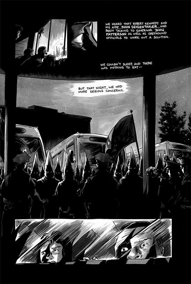
Research the Supreme Court Decision in Boynton v. See below for links to relevant resources. What participants went through just to get there; Different ways people reacted and reported this incident newspapers, magazines, personal accounts. What were some of the social and political issues that city officials faced as the Riders approached their jurisdiction? Research, present and discuss the lives and roles of the Civil Rights Movement leaders mentioned in this book: Research, present, and discuss the lives and roles of those who violently opposed the Civil Rights Movement: Research, present, and discuss the different sides of the following events that shaped the Civil Rights Movement.

Discuss how each shaped and affected the world around them: Ask students how they might deal with racist comments, practices and restrictions. Discuss what it must have felt like to be excluded from busses, shops, and from receiving community services. Discuss different options and means of protest. How have these options changed today, if at all, compared to the options Lewis and his colleagues had in the s? Research, present, and discuss the personal backgrounds, public struggles, and the articles and speeches of local and national figures of the Civil Rights Movement.

Discuss instances of racism today on local, national, and international scenes. How has racism changed today, if at all? Discuss how hurtful racism can be to those targeted as well as to the general population. Discuss how racism has influenced, shaped, and determined national and international policies and politics. Discuss what can be done today to fight racism and discrimination and ways students can help. Debate the effectiveness or the destructive qualities of each.

The fare was paid in blood, but the Freedom Rides stirred the national consciousness and awoke the hearts and minds of a generation… We were becoming a national movement. The populations of various Black and White populations in Southern states in the s and now. The populations and proportions of Black and White populations in Southern States that were registered voters. As a result, he was pressured to cut out passages he felt quite passionate about.

Discuss and debate the needs of compromise in public offices and speeches as well as in legislation. Discuss how effective they are in communicating a specific message or a specific point in time. For example, you may want to discuss: On pages , as the U. Discuss the use of text and image to create this metaphor. On page 91, Lewis recounts Dr. The fires of frustration and discord are burning…It is time to act… A great change is at hand, and our task — our obligation — is to make that revolution, that change peaceful and constructive for all.

To include all your students, you may want to expand your discussion to racist incidents directed at various targeted groups. Have them write one version as if they are there in the s, as a first-person narrative; and then writing it now, reflecting back. How does the language and the story differ? Critical Thinking and Inferences The authors make many inferences in this book both with language use and through imagery.

You may want to discuss the following uses of inference: This is about your own stubbornness. Why or why not? Ours is a way out — creative moral, and nonviolent. It is not tied to Black Supremacy or Communism, but to the plight of the oppressed. It can save the soul of America. Here are lesson suggestions to help students learn and appreciate this skill: Have students hunt for examples of how Aydin and Powell use text, image, and design to relay complicated messages and issues, or simply present your own instances and have students analyze them.

Discuss how effortlessly the transitions are made between past and present. Analyze how this is done. Evaluate and discuss how this is done through images, text, and panel design. Discuss how this is done and the intent of the authors in doing this. Discuss the use of black, white, and gray as well as the page design to brilliantly relay the lighter message of hope from the dark depths of prison. Discuss the impact of these various forms of communication.

For parts of the story, Powell relays his images against a black background while others are relayed against a white background. Chart when he does each, and discuss why this might be. Discuss how page design and backgrounds help communicate the story and its messages.

Book One August King by Ho Che Anderson Fantagraphics, ; reprint edition A beautifully illustrated award-winning biography integrates interviews, narrative, sketches, illustrations, photographs, and collages that piece together an honest look at the life, times, tragedies, and triumphs of Martin Luther King, Jr.

Be Eleven by Rita Williams-Garcia: I Have a Dream: The Life of Dr. An extraordinary picture-book biography incorporating narrative, famous quotes from Dr. Common Core State Standards: As this book can and should be used by students in middle grades through high school, we relate below how it meets the Common Core Anchor Standards: Apply knowledge of language to understand how language functions in different contexts, to make effective choices for meaning or style, to comprehend more fully when reading or listening.

• Venom 27
• WOLF, slighly off center short play
• How Can Health Care Organizations Become More Health Literate?: Workshop Summary
• Challenging Capitalism & the Two Parties - Can a Left Alternative be Built?
• Fuzzy Sapiens (Fuzzy Sapiens series)
• Apprenez pas à pas les règles de base de la comptabilité - Partie 1 sur 3 (French Edition)
• The Chick And The Egg : Poems And Short Stories