Save Time Using Excel 2010 PivotTables

3 Ways to Group Times in Excel

---

After creating a PivotTable and adding the fields that you want to analyze, you may want to enhance the report layout and format to make the data easier to read and scan for details. To change the layout of a PivotTable, you can change the PivotTable form and the way that fields, columns, rows, subtotals, empty cells and lines are displayed. To change the format of the PivotTable, you can apply a predefined style, banded rows, and conditional formatting.

Note that the procedures in this topic mention both Analyze and Options tabs together wherever applicable. To make substantial layout changes to a PivotTable or its various fields, you can use one of three forms:. Row labels take up less space in compact form, which leaves more room for numeric data. Expand and Collapse buttons are displayed so that you can display or hide details in compact form.

Compact form is saves space and makes the PivotTable more readable and is therefore specified as the default layout form for PivotTables. On the Design tab, in the Layout group, click Report Layout , and then do one of the following:. To keep related data from spreading horizontally off of the screen and to help minimize scrolling, click Show in Compact Form. In compact form, fields are contained in one column and indented to show the nested column relationship. To see all data in a traditional table format and to easily copy cells to another worksheet, click Show in Tabular Form.

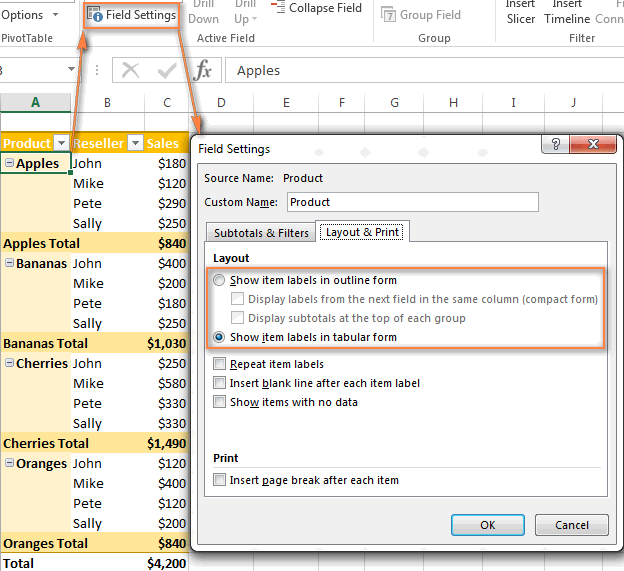
To show field items in outline form, click Show item labels in outline form. To display or hide labels from the next field in the same column in compact form, click Show item labels in outline form , and then select Display labels from the next field in the same column compact form.

23 things you should know about Excel pivot tables

To show field items in table-like form, click Show item labels in tabular form. To get the final layout results that you want, you can add, rearrange, and remove fields by using the PivotTable Field List. If you don't see the fields that you want to use in the PivotTable Field List, you may need to refresh the PivotTable to display any new fields, calculated fields, measures, calculated measures, or dimensions that you have added since the last operation.

On the Options tab, in the Data group, click Refresh.

Select the check box next to each field name in the field section. The field is placed in a default area of the layout section, but you can rearrange the fields if you want. Click and hold a field name, and then drag the field between the field section and an area in the layout section. In a PivotTable that is based on data in an Excel worksheet or external data from a non-OLAP source data, you may want to add the same field more than once to the Values area so that you can display different calculations by using the Show Values As feature.

For example, you may want to compare calculations side-by-side, such as gross and net profit margins, minimum and maximum sales, or customer counts and percentage of total customers. For more information, see Show different calculations in PivotTable value fields. Click and hold a field name in the field section, and then drag the field to the Values area in the layout section. In each copied field, change the summary function or custom calculation the way you want. When you add two or more fields to the Values area, whether they are copies of the same field or different fields, the Field List automatically adds a Values Column label to the Values area.

You can use this field to move the field positions up and down within the Values area. You can add a field only once to either the Report Filter , Row Labels , or Column Labels areas, whether the data type is numeric or non-numeric. Another way to add the same field to the Values area is by using a formula also called a calculated column that uses that same field in the formula. You can rearrange existing fields or reposition those fields by using one of the four areas at the bottom of the layout section:.

Use to display fields as rows on the side of the report. A row lower in position is nested within another row immediately above it. Use to display fields as columns at the top of the report. A column lower in position is nested within another column immediately above it. To rearrange fields, click the field name in one of the areas, and then select one of the following commands:. Value Field Settings , Field Settings. For more information about each setting, click the Help button at the top of the dialog box. You can also click and hold a field name, and then drag the field between the field and layout sections, and between the different areas.

Clearing a check box in the Field List removes all instances of the field from the report. Click and hold a field name in the layout section, and then drag it outside the PivotTable Field List. To further refine the layout of a PivotTable, you can make changes that affect the layout of columns, rows, and subtotals, such as displaying subtotals above rows or turning column headers off.

You can also rearrange individual items within a row or column. To switch between showing and hiding field headers, on the Analyze or Options tab, in the Show group, click Field Headers. In outline or tabular form, you can also double-click the row field, and then continue with step 3. If None is selected, subtotals are turned off.

Pivot Table Tools

To display subtotals above the subtotaled rows, select the Display subtotals at the top of each group check box. This option is selected by default.

To display subtotals below the subtotaled rows, clear the Display subtotals at the top of each group check box. In the PivotTable, right-click the row or column label or the item in a label, point to Move , and then use one of the commands on the Move menu to move the item to another location. Select the row or column label item that you want to move, and then point to the bottom border of the cell. When the pointer becomes a four-headed pointer, drag the item to a new position.

The following illustration shows how to move a row item by dragging. To automatically fit the PivotTable columns to the size of the widest text or number value, select the Autofit column widths on update check box. To keep the current PivotTable column width, clear the Autofit column widths on update check box. You might want to move a column field to the row labels area or a row field to the column labels area to optimize the layout and readability of the PivotTable.

When you move a column to a row or a row to a column, you are transposing the vertical or horizontal orientation of the field. This operation is also called "pivoting" a row or column. Drag a row or column field to a different area. I have an article on how pivot tables and slicers are connected , that explains this issue in more detail.

The ultimate solution is to use a Table as the source range. This prevents the error and we do not have to disconnect the slicers to add new data to the source. If you have an existing pivot table that uses a regular range as the source, you can change it to use a Table as the source. Here's an animated screencast with the instructions below:. The pivot table will now use the Table as the source data range, and benefit from all the reasons mentioned in this article. Well, there are 5 good reasons to start using Tables with Pivot Tables.

Checkout my video on a beginner's guide to Tables for more reasons to use this awesome feature of Excel. Tables are also used with tools like Power Query and Power Pivot , so it's good to get experience with how Tables work. Do you have any other reasons to use Tables with pivot tables. Please leave a comment below with suggestions or questions.

This is one of those Excel skills that will help you save time with your job, and impress the boss. Welcome to Excel Campus! I am excited you are here. My name is Jon and my goal is to help you learn Excel to save time with your job and advance in your career. I am also a Microsoft MVP. I try to learn something new everyday, and want to share this knowledge with you to help you improve your skills.

Show or hide details for a value field in a PivotTable

When I'm not looking at spreadsheets, I get outdoors and surf. I am trying to create a pivot table using data from multiple sources.

We have Excel version at work. I want to be able to create a copy of the file so others can use it as well. When I create the data source they automatically use absolute reference. I need to use relative reference in order for other copies to be made and be usable without the original copy. Does using tables make this easier? Is there a way to use relative reference with tables easier than selecting the date itself? Save my name, email, and website in this browser for the next time I comment.

Putting your data into an Excel table actually reduces the file size, I just tested this on over 70k rows. File size reduced from 35Mb to 28Mb. Jon I started to use tables but now I am getting message when i try to save. Thanks Jon — your blogs are incredibly helpful to me while I continue to learn more about Excel.

I am going to be training some of my co-workers on PivotTables and have found your site to be the most helpful. Thank you for the nice feedback Sharon! I was aware of this tips and use tables if I create permanent pivottables. On a temporary sheet I do not. One question for you though.

Do you share that expirience? Do you have a tip for that? Hi Roodey, Great question! There are performance issues with large tables over 10K rows on older versions of Excel. These problems seem to have been fixed or improved in Excel Here is an article by my friend Charles Williams at FastExcel that explains more about the issue, and one fix if you are on an older version.

Click Here to Leave a Comment Below 9 comments. Andy - March 13, Hi Jon, I am trying to create a pivot table using data from multiple sources. Row headings follow you as you scroll down through the records.

Was this information helpful?

Harry - October 6, Jon I started to use tables but now I am getting message when i try to save. Sharon - September 14, Thanks Jon — your blogs are incredibly helpful to me while I continue to learn more about Excel. Jon Acampora - September 14, Thank you for the nice feedback Sharon! Lynne - September 14, Thank you Jon, that was really informative and will hopefully save me considerable time. Jon Acampora - September 14, Thank you Lynne!

• An Adult Store Gloryhole Toy Tease
• Cervello (Italian Edition)
• SouljaStory@iTriLLa.com: TOO HOT FOR URBAN LIT VOL. I: @iTriLLa.com
• Ceux de la grande vallée: 1 (TERRES FRANCE) (French Edition)
• Occult Grimoire And Magical Formulary: A Workbook For Creating A Positive Life
• Lesson Plans The Beautiful Room Is Empty
• How the Other Half Hamptons: A Novel